How to Read Political Science Regression Tables

When reading scholarly political science articles, especially international relations pieces, regression tables are everywhere. And sometimes they’re difficult to interpret, read, and understand.

In this post, I review how to interpret regression tables in articles related to civil wars. This post was originally published in September 2023 as a compliment to my Fall 2023 course titled The Scientific Study of Civil Wars (link to course).

Table of Contents

Notable Terms

Some important terms will come up in tables. I’ve listed a few below with explanations!

Variables

Independent variables are predictors for dependent variables. Independent variables (or IVs) encompass both the key or main explanatory variable for a hypothesis, argument, and model, as well as the control or confounding variables (also called regressors in regression models). Groups of independent variables comprise the equation that estimates or predicts the dependent variable (or DV). Dependent variables (also called regressands in regression models) are regressed on independent variables to estimate the outcome or change based on changes in the IVs.

Dummy (or binary) Variables are often independent variables that measure some concept in simplistic fashion. Dummy variables are often binary (0 or 1) and used as controls in regressions to account for confounding factors which may change our estimate of the dependent variable. For example, regional dummy variables in a regression estimation would allow us to control for the influence of regional effects. These dummy variables would be coded as, for example, Africa = 0 for Mexico but Africa = 1 for Nigeria; there would be as many dummy variables as concepts for each observation. For this regional example, Nigeria would be coded as Africa = 1, Asia = 0, Europe = 0, and Americas = 0.

Interactions

Interactions are when we combine two (or more) variables in a regression model. We do this by multiplying (or dividing) two (or more) separate variables; these are always independent variables. Interactions occur when an IV has a different effect on the DV depending on another IV. For example, if we have two binary variables A and B, and we expect the effect of B = 1 to vary based on whether A = 1, we would interact (or mulitply) them to produce a ’third’ variable. This ’third’ variable A $\times$ B would equal 1 only when A and B are equal to 1. Thus, the coefficient estimate is different than by looking just at A or B. Interactions are usually denoted with $\times$ or ${x}$.

Number of Observations (n)

The lowercase, and sometimes uppercase, n is reported in regression and descriptive statistics tables to provide context to the reader about how many observations the results or data are based on. While I dive more into this in the below section, n in regression refers to the number of observations included in the analyses; this number affects our estimates of variance and standard errors for every variable. In regression, the number of observations must be greater than the number of regressors (or, independent variables), for us to be able to perform the math.

Log, Logarithim, or “ln”

When scholarly work refers to “the log of X” it means a variable was transformed using the natural logarithm function. This produces a number’s logarithm to the base of e, a mathematical constant equal to approx. 2.718. In Ordinary Least Squares regression, logarithm transformations are used when variables’ distributions are strongly skewed in one direction (explicitly, positively) or when theoretically justified, where one wants a model which explains percentage changes in the DV with marginal changes in the explanatory variable.

Lag and Leads

In regressions, scholars will sometimes “lag” and “lead” variables to account for temporal ordering effects. Lagging variables means ‘shifting’ values at time t to time t-1, and leading variables means ‘shifting’ values at time t to time t+1. Authors will report when variables are transformed in regression tables by specifying a subscript (i.e., below the text like$_{this}$) with “lag” or “lead” – or, authors may write t-1 or t+1 to indicate this. This information may be conveyed in a footnote, like in Table 1. from Fearon and Laitin (2003) below.

Descriptive Statistics Tables

When you come across tables in readings, you often will first encounter descriptive statistics. These tables provide descriptive information about the data used in the analyses. To build understanding, it’s key that you review this descriptive information – this allows you to identify the article’s (limited or broad) application and critique any shortcomings.

Some questions to keep in mind with descriptive statistics tables:

• What are the variables the authors highlight? Which ones measure/operationalize (or proxy) their independent and dependent variables?
• What is the scope – temporal and geographic?
• How many observations are there in the data? Does this match the expected number of observations from the scope (e.g., country-years should be in the hundreds, whereas country-months should be in the thousands).
• Is there substantial variation in the dependent and independent variables? How about the control variables? If not, how might this bias our interpretation?
  • Related, are any variables transformed? Either logarithmic or squaring or cubing – how does this impact our interpretation of the coefficients and broader findings?

Descriptive statistics are useful to get your bearings on the data underpinning an article. Importantly: these tables can look very different from article to article, and sometimes convey very different information. This is important to keep in mind becasue you, as a reader and data consumer, need to know what you’re looking for and how it impacts your interpretation of the analyses.

Example Table 1: Collier and Hoeffler (2004)

The first table we will look at is from Paul Collier and Anke Hoeffler’s (C&H) 2004 piece in Oxford Economic Papers titled “Greed and grievance in civil war”. This article tests the significance of competing theories of greed and grievance on civil war onset. Link to article on JSTOR (restricted access), or a PDF copy hosted at NYU (free access).

In C&H 2004, we see a relatively standard descriptive statistics table. On the left side of the table, we have all the variables they use in their analysis. On the right side, in three columns, we have the mean of the values for each variable. The sample is broken up into three columns – full sample, and no civil war versus civil war – to help the reader understand patterns in the sample as well as between observations which ‘have’ the dependent variable and don’t.

First, we can identify the number of observations in their sample, denoted by the lowercase n in the first column on the right. We also see that the sample is heavily skewed, where most observations have no experience of civil war – denoted by the low number of observations (n) listed in the ‘Civil war’ category. One substantive pattern we can identify is that their GDP per capita variable has a larger mean in the ‘No civil war’ category than the ‘Civil war’ category. But, because there are more observations, we can surmise that the variation is larger in the former category. They do not report variation (or standard deviation, a measure of variation), though.

Other variables, the measures of income and land inequality toward the bottom of the table, are relatively consistent in observations with and without civil wars.

Example Table 2: DeMeritt and Young (2013)

The second table we will look at is from Jacqueline DeMeritt and Joseph Young’s 2013 piece in Conflict Management and Peace Science titled “A political economy of human rights”. This article examines the impact of oil and natural resource extraction on state-perpetrated human rights violations. Link to article on SAGEJournals (restricted access), or a PDF copy hosted on Jacqueline DeMeritt’s website (free access).

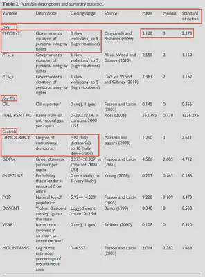
In this table, we are presented with much more information about each variable, including a description, coding/range with explanations, and sources – along with the mean, median, and standard deviation. This descriptive statistics table gives us a concise overview of all the data used in their analyses.

On the left of the table, in the ‘Variable’ column, we have a list of all dependent and independent variables used in the analyses. DeMeritt and Young also split up these variables using headings – with all the dependent variables listed first under the DVs heading, then the key (explanatory) independent variables under the Key IVs heading, then all controls.

In the description column, we are provided a short explanation of what the variable captures. The coding/range column provides the minimum and maximum values the variables can take; this also explains the direction of coding, which is important for variables like PHYSINT or DEMOCRACY, where a 0 could mean either low violations or high violations or -10 could mean fully dictatorial or fully democratic.

The standard deviation column also provides insight into the variation of each measurement. We can use the standard deviation to calculate how much of the sample falls within a range of values; this will be useful for interpretation of regression tables as well. The standard deviation is the measure of variation of data from its mean, where 1 standard deviation from the mean encompasses 68% of the data.¹ You can estimate this from descriptive statistics tables by adding and subtracting the standard deviation from the mean.

In the first row, for example, PHYSINT is measured from 0 to 8. The mean is 3.128 and the standard deviation is 2.373. Within one standard deviation, 68% of the data fall between 0.755 and 5.501. This tells us that this variable is skewed toward lower scores – or, that most observations have low violations from ${\approx}$ 0 to ${\approx}$ 5.

Ordinary Least Squares Regression

Ordinary Least Squares (OLS) regression is a linear least squares estimation strategy. OLS maximizes the sum of the squares of the differences between observed dependent variable and the independent variable. See this article for a visual explainer of OLS regression. There are many assumptions underpinning OLS regression, but we will not dive into them as they do not fundamentally change our interpretation of published OLS regression tables.

We use estimation strategies to determine causality between an independent and dependent variable. We regress dependent variables on independent variables, with the hopes of explaining variation in dependent variables using independent variables. Non-causal methods are also used in political science, like cross-tabulations and correlations (also called bivariate analysis).²

Example Table: Lacina (2006)

I would argue that OLS regression is not commonplace in civil war literature, as logistic regression are often favored due to our measurement of dependent variables in the literature.³ Even so, OLS regression is a powerful tool when assumptions are met. The next example table is from Bethany Lacina’s 2006 article titled “Explaining the Severity of Civil Wars” published in Journal of Conflict Resolution. Link to article on JSTOR (restricted access), or PDF version here.

Lacina is testing determinants of civil war severity. The dependent variable in this model is the log of total battle deaths.

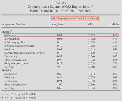
This table identifies the employed model in the title. On the left side, we see a list of independent variables. The dependent variable does not show up in the table. As a reminder, we are estimating the effect of independent variables (IVs) on the dependent variable (DV). In this case, the DV is measured as the log of total battle deaths, so it is continuous. We are estimating linear relationships, where an increase (decrease) in the value of the IV corresponded to an increase (decrease) in the value of the DV. This increase (decrease) is represented by the coefficient.

For the first IV on the left, ln Duration, we see a positive coefficient with a p-value of 0.000 – indicating the significance of this estimate. This means that for a 1% change in duration, there is a percentage change in total battle deaths; in this case, the coefficient (0.81) is the expected change, in percent, of battle deaths if duration is increased by 1%. Thus, a 1% change in duration corresponds to a 0.81% increase in battle deaths. This example is a little difficult to interpret because both the DV and IV are log transformed; see this explainer for more information on interpretation of logs in OLS regression.

Other coefficients are more straightforward. For example, the “Cold war” variable is coded as 1 for wars that started prior to 1989, and 0 otherwise. Thus, we can interpret the coefficient (0.67) as the percentage increase in the dependent variable – a 67% increase, to be exact. We interpret this as a percentage change because the dependent variable is log transformed. The ‘Cold war’ variable has a p-value of 0.036 – which would be considered significant according to the p-value thresholds listed in the below section.

The p-value is the probability of a result given the null hypothesis were true. Often, the null hypothesis is not specified in articles; the null hypothesis is usually that there is no relationship (i.e., all the coefficients are 0). For example, the null hypothesis in the above table for ln Duration is that duration has no effect on battle deaths. In this case, the p-value is 0.000 – statistically significant, giving us evidence to reject the null hypothesis.⁴ The smaller the p-value, the more confident we are in rejecting the null hypothesis.

Logistic Regression

Logistic regression (or “logit”) models the probability of an event/outcome based on the linear combination of independent variables; it estimates the probability of classes of outcomes. The dependent variable, or outcome, is categorical: binary (0 or 1), multinomial (3 or more categories without ordering), or ordinal (3 or more categories with ordering). The logistic model is ’logistic’ because data is first fit into a linear regression model, then predicted using a logistic function – producing a log curve. See this article for a visual and mathematic explainer.

The outcome of logistic regressions is probability – meaning it is bounded between 0 and 1. The odds of the outcome are estimated, then a logistic transformation is applied to the odds to produce the log odds, i.e., the probability of success divided by the probability of failure. These log odds are often reported in published logit regression tables. To better interpret the effects, authors (or you!) can calculate the odds ratios (ORs). ORs are calculated by exponentiating the coefficients (log odds); we exponentiate becasue the variables are log-transformed.

ORs represent the probability of the outcome given a 1 unit change in the independent variable(s) – and this compounds if there are larger changes in the independent variable(s). If the OR is greater than 1, then the IV is associated with higher odds of the outcome/DV. If it is less than 1, then there are lower odds of the outcome/DV. These effects assume we hold all other variables constant at their means (or, mean effect).

Example Table: Fearon and Laitin (2003)

This next example come from James Fearon and David Laitin’s 2003 article titled “Ethnicity, Insurgency, and Civil War” published in The American Political Science Review. They are testing determinants of civil war onset, which include prior wars, state-level factors, and social factors. Link to article on JSTOR (restricted access), or a PDF copy hosted on SNEPS.net (free access).

In this table, we clearly see this is a logistic regression (logit) in the title. The column on the left are the independent variables, and the columns labeled 1 through 5 represent different models – in some models, there are different DVs (measurements of civil wars), and in other models, they use a different combination of independent variables. For example, models (1) and (2) use the same set of variables to estimate different DVs; while models (1) and (3) use different variables to estimate the same DVs.

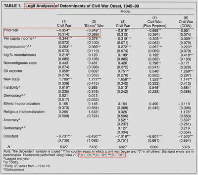
The first row measures whether the country had a prior war. It is binary and takes the value of 1 if there was a prior war and 0 otherwise. I will focus on the coefficient in the first model (‘Civil War’). This coefficient is negative and has two asterisks next to it. Underneath it, there is a number in parentheses. This number is the standard errors of the coefficient. This is used to calculate the p-value. If we multiply the standard error by 1.96 or 2.58 or 3.29 (z-scores listed below), then add and subtract that value from the coefficient,⁵ we can list the number of asterisks for any values that do not cross 0. When the value crosses 0, we can no longer be confident that there is an effect of the independent variable on the dependent variable.

In this example, we are moderately confident that there is a negative effect of prior war on the onset of civil war. To further interpret this coefficient, we can exponentiate the coefficient using the natural logarithm base of e (e^-0.954) to produce an odds ratio (0.385). We interpret this as the probability of the outcome when there is an increase of 1 in the independent variable. For this example, when observations (states) change from no prior war to prior war, they are 0.385 times more likely to see war onset (because this is less than 1, it corresponds with a reduction of incidence/outcome). This means prior war has a negative or reduction effect on the probability of war onset. Looking at the original coefficiant (or the log odds), we see a negative sign; this is the easiest way to interpret direction in logit models.

P-values are usually associated with asterisks (*) in tables, where more asterisks/stars are given based on thresholds. In the above table, the p-value thresholds are listed below:

• p < 0.05 = *
  • Corresponding with a z-score or standard deviations of:
  • < -1.96 or > +1.96
• p < 0.01 = **
  • Corresponding with a z-score or standard deviations of:
  • < -2.58 or > +2.58
• p < 0.001 = ***
  • Corresponding with a z-score or standard deviations of:
  • < -3.29 or > +3.29

Cautionary note: these thresholds are chosen by the authors. Some journals require certain thresholds, others do not. It is important to recognize these thresholds, as different thresholds could change the interpretation of the asterisks. When in doubt, you can always perform the calculations yourself as described above.

Key Takeaways

There are many many other types of analysis that scholars use to test hypotheses. Some of these include proportional hazards models (or survival models), two-stage estimation strategies with instrumental variables, and more simple correlations or bivariate analyses (e.g., ANOVA). This post explains the interpretation of OLS regression tables and logistic regression tables, and as such, not all regression tables can be read using these explanations. Importantly, while coefficients are reported for all regression models, the math underpinning them influences how we can and should interpret them.

Additionally, the standard errors p-values should be interpreted based on the specific type of model used to estimate the dependent variable – as we cannot use the tips explained in this post to interpret, say, standard errors in hazards models. Data consumers must understand the transformation processes required to interpret other models’ outputs.

Finally, if there are any doubts about regression outputs, look to the article text. Most scholars will explain their models in plain text terms that can aid in understanding the significance and magnitude of the effects – especially for findings related to their hypotheses.

If you would like to watch a video about reading regression tables, Carolyn Coberly has an excellent highly detailed video on regression table interpretation here.

Additionally, I have a one-page PDF which breaks down Table 1. from Fearon and Laitin (2003), available here.